Laws of Return to Scale

“The term returns to scale refers to the changes in output as all factors change by the same proportion.” – Koutsoyiannis

“Returns to scale relates to the behaviour of total output as all inputs are varied and is a long run concept”.  Leibhafsky

It is important to realize that the study of production completely differs according to the time frame. Recollect that we take the help of the law of diminishing returns to study production in the short run, whereas in the long run, the returns to scale are at the helm.

Again, the long run is a long enough period in which we can alter both fixed and variable factors. Thus, in the long run, we aim to study the effect of the changes in all the inputs on the production output.

However, these changes are not random. All the factors are increased or decreased together. This is also known as changes in scale, hence the name return to scale.

Thus, in the long run, we proportionately vary the inputs and observe the relative change in production. Of course, the return to scale can be of three types- increasing, decreasing and constant

Returns to scale are of the following three types

1. Increasing Returns to scale.
2. Constant Returns to Scale
3. Diminishing Returns to Scale

In the long run, output can be increased by increasing all factors in the same proportion. Generally, laws of returns to scale refer to an increase in output due to increase in all factors in the same proportion. Such an increase is called returns to scale.

Suppose, initially production function is as follows:

P = f (L, K)

Now, if both the factors of production i.e., labour and capital are increased in same proportion i.e., x, product function will be rewritten as.

The above stated table explains the following three stages of returns to scale:

1. Increasing Returns to Scale

Increasing returns to scale or diminishing cost refers to a situation when all factors of production are increased, output increases at a higher rate. It means if all inputs are doubled, output will also increase at the faster rate than double. Hence, it is said to be increasing returns to scale. This increase is due to many reasons like division external economies of scale. Increasing returns to scale can be illustrated with the help of a diagram 8.

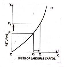
In this figure , OX axis represents increase in labour and capital while OY axis shows increase in output. When labour and capital increases from Q to Q₁, output also increases from P to P₁ which is higher than the factors of production i.e. labour and capital.

2. Diminishing Returns to Scale

Diminishing returns or increasing costs refer to that production situation, where if all the factors of production are increased in a given proportion, output increases in a smaller proportion. It means, if inputs are doubled, output will be less than doubled. If 20 percent increase in labour and capital is followed by 10 percent increase in output, then it is an instance of diminishing returns to scale.

The main cause of the operation of diminishing returns to scale is that internal and external economies are less than internal and external diseconomies. It is clear from diagram 9.

In this diagram, diminishing returns to scale has been shown. On OX axis, labour and capital are given while on OY axis, output. When factors of production increase from Q to Q₁ (more quantity) but as a result increase in output, i.e. P to P₁ is less. We see that increase in factors of production is more and increase in production is comparatively less, thus diminishing returns to scale apply.

3. Constant Returns to Scale

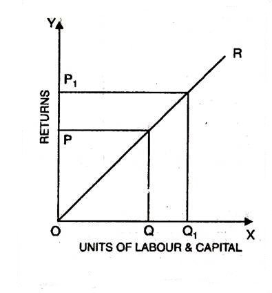
Constant returns to scale or constant cost refers to the production situation in which output increases exactly in the same proportion in which factors of production are increased. In simple terms, if factors of production are doubled output will also be doubled.

In this case internal and external economies are exactly equal to internal and external diseconomies. This situation arises when after reaching a certain level of production, economies of scale are balanced by diseconomies of scale. This is known as homogeneous production function. Cobb-Douglas linear homogenous production function is a good example of this kind. This is shown in diagram. In figure, we see that increase in factors of production i.e. labour and capital are equal to the proportion of output increase. Therefore, the result is constant returns to scale.

CONSTANT RETURNS TO SCALE

For constant returns to scale to occur, the relative change in production should be equal to the proportionate change in the factors.

For example, if all the factors are proportionately doubled, then constant returns would imply that the production output would also double. Interestingly, the production function of an economy as a whole exhibits close characteristics of constant returns to scale.

Also, studies suggest that an individual firm passes through a long phase of constant return to scale in its lifetime. Lastly, it is also known as the linear homogeneous production function.

INCREASING RETURNS TO SCALE

Here, the proportionate increase in production is greater than the increase in inputs. Note that upon expansion, a firm experiences increasing returns to scale. The indivisibility of factors is another reason for this.

Some factors are available in large units, such that they are completely suitable for large-scale production. Evidently, if all the factors are perfectly divisible then there might be no increasing returns. Further, specialization of land and machinery can be another reason.

DECREASING RETURNS TO SCALE

An incidence of decreasing returns to scale would mean that the increase in output is less than the proportionate increase in the input. Generally, this happens when a firm expands all its inputs, especially a large firm.

When the firm expands to a very large size, it becomes difficult to manage it with the same efficiency as before. Hence, the increasing complexity in management, coordination, and control eventually leads to decreasing returns.

Cobb Douglas Production Function

The Cobb Douglas production function {Q(L, K)=A(L^b)K^a}, exhibits the three types of returns:

• If a+b>1, there are increasing returns to scale.
• For a+b=1, we get constant returns to scale.
• If a+b<1, we get decreasing returns to scale.