 by
by In economics, economic equilibrium is a situation in which economic forces such as supply and demand are balanced and in the absence of external influences the (equilibrium) values of economic variables will not change. For example, in the standard text perfect competition, equilibrium occurs at the point at which quantity demanded and quantities supplied are equal.
Market equilibrium in this case is a condition where a market price is established through competition such that the amount of goods or services sought by buyers is equal to the amount of goods or services produced by sellers. This price is often called the competitive price or market clearing price and will tend not to change unless demand or supply changes and quantity is called the “competitive quantity” or market clearing quantity. But the concept of equilibrium in economics also applies to imperfectly competitive markets, where it takes the form of a Nash.
Properties of equilibrium
Three basic properties of equilibrium in general have been proposed by Huw Dixon. These are:
Equilibrium property P1: The behavior of agents is consistent.
Equilibrium property P2: No agent has an incentive to change its behavior.
Equilibrium property P3: Equilibrium is the outcome of some dynamic process (stability).
Types of Economic Equilibrium
Microeconomics
Microeconomics is concerned with individuals’ and businesses’ activities and how they interact to achieve maximum results. Here, economic equilibrium occurs when the price of a good is equal to satisfying supply and demand needs.
When supply and demand intersect, this is considered the point of economic equilibrium, and the price is determined accordingly. The Apple example from above can be seen as a case of microeconomic equilibrium.
Macroeconomics
Macroeconomics looks at the economy from a wider lens. It involves studying economic factors like gross domestic product (GDP), interest rates, and fiscal spending. Economic equilibrium is achieved in macroeconomics by balancing the inputs and outputs, such as aggregate demand and aggregate supply.
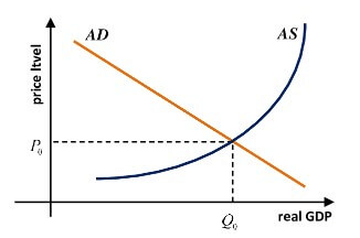
When an economy can match the nation’s aggregate supply and aggregate demand, it is in economic equilibrium. If the economy has more supply than demand, it is wasting resources. However, if they have more demand than supply, they miss out on profits.
Static vs. Dynamic
The economic equilibrium in micro and macroeconomics can be further divided into static and dynamic categories.
Static = In static equilibrium, the factors or inputs will not change. For example, demand and supply will remain constant. As a result, all parties involved are achieving maximum gratification.
Dynamic = In dynamic equilibrium, the factors or inputs are constantly varying. Examples can include prices, rates, and ever-changing income levels.
Competitive equilibrium
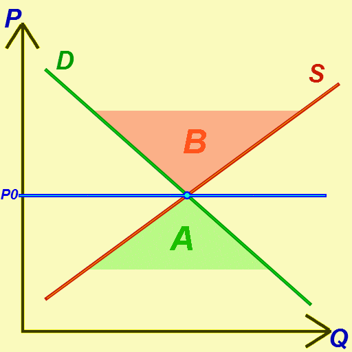
P – price
Q – quantity demanded and supplied
S – supply curve
D – demand curve
P0 – equilibrium price
A – excess demand – when P<P0
B – excess supply – when P>P0
In a competitive equilibrium, supply equals demand. Property P1 is satisfied, because at the equilibrium price the amount supplied is equal to the amount demanded. Property P2 is also satisfied. Demand is chosen to maximize utility given the market price: no one on the demand side has any incentive to demand more or less at the prevailing price. Likewise supply is determined by firms maximizing their profits at the market price: no firm will want to supply any more or less at the equilibrium price. Hence, agents on neither the demand side nor the supply side will have any incentive to alter their actions.
To see whether Property P3 is satisfied, consider what happens when the price is above the equilibrium. In this case there is an excess supply, with the quantity supplied exceeding that demanded. This will tend to put downward pressure on the price to make it return to equilibrium. Likewise where the price is below the equilibrium point there is a shortage in supply leading to an increase in prices back to equilibrium. Not all equilibria are “stable” in the sense of equilibrium property P3. It is possible to have competitive equilibria that are unstable. However, if an equilibrium is unstable, it raises the question of reaching it. Even if it satisfies properties P1 and P2, the absence of P3 means that the market can only be in the unstable equilibrium if it starts off there.
Nash equilibrium

The Nash equilibrium is widely used in economics as the main alternative to competitive equilibrium. It is used whenever there is a strategic element to the behavior of agents and the “price taking” assumption of competitive equilibrium is inappropriate. The first use of the Nash equilibrium was in the Cournot duopoly as developed by Antoine Augustin Cournot in his 1838 book. Both firms produce a homogenous product: given the total amount supplied by the two firms, the (single) industry price is determined using the demand curve. This determines the revenues of each firm (the industry price times the quantity supplied by the firm). The profit of each firm is then this revenue minus the cost of producing the output. Clearly, there is a strategic interdependence between the two firms. If one firm varies its output, this will in turn affect the market price and so the revenue and profits of the other firm. We can define the payoff function which gives the profit of each firm as a function of the two outputs chosen by the firms. Cournot assumed that each firm chooses its own output to maximize its profits given the output of the other firm. The Nash equilibrium occurs when both firms are producing the outputs which maximize their own profit given the output of the other firm.
In terms of the equilibrium properties, we can see that P2 is satisfied: in a Nash equilibrium, neither firm has an incentive to deviate from the Nash equilibrium given the output of the other firm. P1 is satisfied since the payoff function ensures that the market price is consistent with the outputs supplied and that each firms profits equal revenue minus cost at this output.
Cournot himself argued that it was stable using the stability concept implied by best response dynamics. The reaction function for each firm gives the output which maximizes profits (best response) in terms of output for a firm in terms of a given output of the other firm. In the standard Cournot model this is downward sloping: if the other firm produces a higher output, the best response involves producing less. Best response dynamics involves firms starting from some arbitrary position and then adjusting output to their best-response to the previous output of the other firm. So long as the reaction functions have a slope of less than -1, this will converge to the Nash equilibrium. However, this stability story is open to much criticism. As Dixon argues: “The crucial weakness is that, at each step, the firms behave myopically: they choose their output to maximize their current profits given the output of the other firm, but ignore the fact that the process specifies that the other firm will adjust its output…”. There are other concepts of stability that have been put forward for the Nash equilibrium, evolutionary stability for example.
Disequilibrium
Disequilibrium characterizes a market that is not in equilibrium. Disequilibrium can occur extremely briefly or over an extended period of time. Typically in financial markets it either never occurs or only momentarily occurs, because trading takes place continuously and the prices of financial assets can adjust instantaneously with each trade to equilibrate supply and demand. At the other extreme, many economists view labor markets as being in a state of disequilibrium specifically one of excess supply over extended periods of ime. Goods markets are somewhere in between: prices of some goods, while sluggish in adjusting due to menu costs, long-term contracts, and other impediments, do not stay at disequilibrium levels indefinitely.
In most simple microeconomic stories of supply and demand a static equilibrium is observed in a market; however, economic equilibrium can be also dynamic. Equilibrium may also be economy-wide or general, as opposed to the partial equilibrium of a single market. Equilibrium can change if there is a change in demand or supply conditions. For example, an increase in supply will disrupt the equilibrium, leading to lower prices. Eventually, a new equilibrium will be attained in most markets. Then, there will be no change in price or the amount of output bought and sold until there is an exogenous shift in supply or demand (such as changes in technology or tastes). That is, there are no endogenous forces leading to the price or the quantity.