Skewness, Concept, Examples, Types and Methods

Skewness, in statistics, is the degree of distortion from the symmetrical bell curve, or normal distribution, in a set of data. Skewness can be negative, positive, zero or undefined. A normal distribution has a skew of zero, while a lognormal distribution, for example, would exhibit some degree of right-skew.

Examples in Real Life

• Positive Skew: Wealth distribution, waiting times in queues, customer complaints.

• Negative Skew: Exam scores when most students perform well, age of retirement, mortgage payoffs.

The three probability distributions depicted below depict increasing levels of right (or positive) skewness. Distributions can also be left (negative) skewed. Skewness is used along with kurtosis to better judge the likelihood of events falling in the tails of a probability distribution.

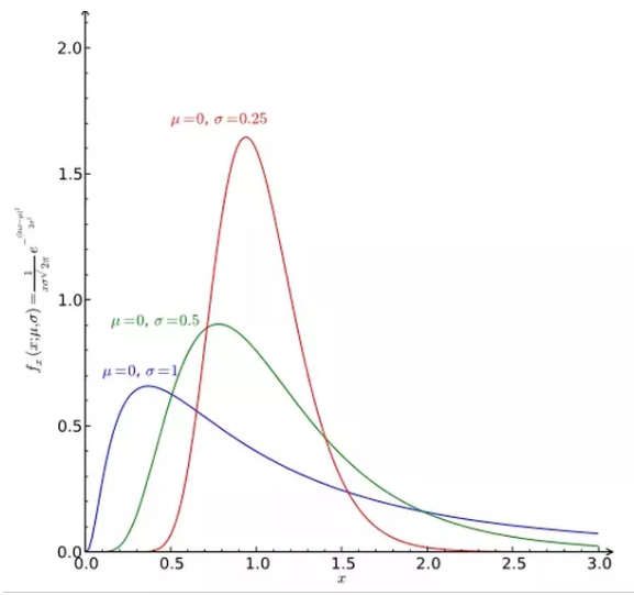
Right skewness

• Skewness, in statistics, is the degree of distortion from the symmetrical bell curve in a probability distribution.
• Distributions can exhibit right (positive) skewness or left (negative) skewness to varying degree.
• Investors note skewness when judging a return distribution because it, like kurtosis, considers the extremes of the data set rather than focusing solely on the average.

Types of Skewness:

1. Positive skewness

A series is said to have positive skewness when the following characteristics are noticed:

• Mean > Median > Mode.
• The right tail of the curve is longer than its left tail, when the data are plotted through a histogram, or a frequency polygon.
• The formula of Skewness and its coefficient give positive figures.

2. Negative skewness

A series is said to have negative skewness when the following characteristics are noticed:

• Mode> Median > Mode.
• The left tail of the curve is longer than the right tail, when the data are plotted through a histogram, or a frequency polygon.
• The formula of skewness and its coefficient give negative figures.

3. Zero Skew (Symmetrical Distribution)

• Both sides of the distribution are mirror images.

• Mean = Median = Mode

• The distribution forms a perfect bell shape (e.g., normal distribution).

Methods of Skewness

1. Karl Pearson’s Coefficient of Skewness

Formula (Using Mode): Skewness = (Mean − Mode) / Standard Deviation​

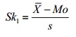
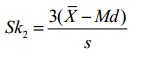
Alternate Formula (Using Median): Skewness = 3(Mean − Median) / Standard Deviation​

Use When:

• Mode is known or can be estimated.

• Data is symmetrical or nearly symmetrical.

Interpretation:

• Sk > 0: Positively skewed

• Sk < 0: Negatively skewed

• Sk = 0: Symmetrical

Example:

If Mean = 65, Median = 60, SD = 10

Sk = 3(65 − 60) / 10 = 15 / 10 = 1.5 (Positive Skew)

2. Bowley’s Coefficient of Skewness

Formula: Sk = (Q3 + Q1 − 2⋅Median) / (Q3 − Q1)​

Where:

• Q1Q_1Q1​ = First Quartile

• Q3Q_3Q3​ = Third Quartile

• Q3−Q1Q_3 – Q_1Q3​−Q1​ = Interquartile Range (IQR)

Use When:

• Dealing with open-ended distributions

• Data contains extreme values/outliers

• Median and quartiles are available instead of mean/mode

Interpretation:

• Sk > 0: Right (positive) skew

• Sk < 0: Left (negative) skew

• Sk = 0: Symmetrical

Example:

If Q1 = 20,  Q3 = 40 and Median = 25

Sk = (40 + 20 − 2(25)) / (40 − 20) = (60 − 50) / 20 = 10 / 20 = 0.5

3. Kelly’s Coefficient of Skewness

Formula: Sk = (P90 + P10 − 2⋅P50) / (P90 − P10)​​

Where:

• P10​, P50, P90​ are 10th, 50th (median), and 90th percentiles

Use When:

• Data is large and detailed

• Analysis requires percentile-based insights

• Quartiles aren’t sufficient

Interpretation:

Same as Bowley’s:

• Sk > 0: Positive skew

• Sk < 0: Negative skew

• Sk = 0: Symmetric distribution

Skewness Co-efficient

• Pearson’s Coefficient of Skewness #1 uses the mode. The formula is:

  Where  = the mean, Mo = the mode and s = the standard deviation for the sample.

• Pearson’s Coefficient of Skewness #2 uses the median. The formula is:

  Where  = the mean, Mo = the mode and s = the standard deviation for the sample.

  It is generally used when you don’t know the mode.