 by
by The law of supply is the microeconomic law that states that, all other factors being equal, as the price of a good or service increases, the quantity of goods or services that suppliers offer will increase, and vice versa. The law of supply says that as the price of an item goes up, suppliers will attempt to maximize their profits by increasing the quantity offered for sale.
Law of supply states that other factors remaining constant, price and quantity supplied of a good are directly related to each other. In other words, when the price paid by buyers for a good rises, then suppliers increase the supply of that good in the market.
Assumptions of the Law of Supply
Important assumptions of the law of supply are as follows:
1. No change in the income
There should not be any change in the income of the purchaser or the seller.
2. No change in technique of production
There should not be any change in the technique of production. This is essential for the cost to remain unchanged. With the improvement in technique if the cost of production is reduced, the seller would supply more even at falling prices.
3. There should be no change in transport cost
It is assumed that transport facilities and transport costs are unchanged. Otherwise, a reduction in transport cost implies lowering the cost of production, so that more would be supplied even at a lower price.
4. Cost of production be unchanged
It is assumed that the price of the product changes, but there is no change in the cost of production. If the cost of production increases along with the rise in the price of product, the sellers will not find it worthwhile to produce more and supply more. Therefore, the law of supply will be valid only if the cost of production remains constant. It implies that the factor prices such as wages, interest, rent etc., are also unchanged.
5. There should be fixed scale of production
During a given period of time, it is assumed that the scale of production is held constant. If there is a changing scale of production the level of supply will change, irrespective of changes in the price of the product.
6. There should not be any speculation
The law also assumes that the sellers do not speculate about the future changes in the price of the product. If, however, sellers expect prices to rise further in future, they may not expand supply with the present price rise.
7. The prices of other goods should remain constant
Further, the law assumes that there are no changes in the prices of other products. If the price of some other product rises faster than that of the product in consideration, producers might transfer their resources to the other product—which is more profit yielding due to rising prices. Under this situation and circumstances, more of the product in consideration may not be supplied, despite the rising prices.
8. There should not be any change in the government policies
Government policy is also important and vital for the law of supply. Government policies like taxation policy, trade policy etc., should remain constant. For instance, an increase in or totally fresh levy of excise duties would imply an increase in the cost or in case there is fixation of quotas for the raw-materials or imported components of a product, then such a situation will not permit the expansion of supply with a rise in prices.
Supply Elasticity; Analysis and its uses for Managerial Decision MakingThe law of supply indicates the direction of change if price goes up, supply will increase. But how much supply will rise in response to an increase in price cannot be known from the law of supply. To quantify such change we require the concept of elasticity of supply that measures the extent of quantities supplied in response to a change in price.
Elasticity of supply measures the degree of responsiveness of quantity supplied to a change in own price of the commodity. It is also defined as the percentage change in quantity supplied divided by percentage change in price.
It can be calculated by using the following formula:
ES = % change in quantity supplied/% change in price
Symbolically,
ES = ∆Q/Q ÷ ∆P/P = ∆Q/∆P × P/Q
Since price and quantity supplied, in usual cases, move in the same direction, the coefficient of ES is positive.
Types of Elasticity of Supply:
For all the commodities, the value of Es cannot be uniform. For some commodities, the value may be greater than or less than one.
1. Elastic Supply (ES>1)
Supply is said to be elastic when a given percentage change in price leads to a larger change in quantity supplied. Under this situation, the numerical value of Es will be greater than one but less than infinity. SS1 curve of Fig. exhibits elastic supply. Here quantity supplied changes by a larger magnitude than does price.
 2. Inelastic Supply (ES< 1)
Supply is said to be inelastic when a given percentage change in price causes a smaller change in quantity supplied. Here the numerical value of elasticity of supply is greater than zero but less than one. Fig. depicts inelastic supply curve where quantity supplied changes by a smaller percentage than does price.
 3. Unit Elasticity of Supply (ES = 1)
If price and quantity supplied change by the same magnitude, then we have unit elasticity of supply. Any straight line supply Curve passing through the origin, such as the one shown in Fig., has an elasticity of supply equal to 1. This can be verified in this way.
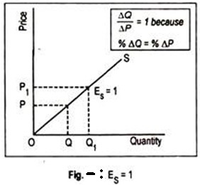
For any straight line positively-sloped supply curve drawn through the origin, the ratio of P/Q at any point on the supply curve is equal to the ratio ∆ P/∆ Q. Note that ∆ P/∆ Q is the slope of the supply curve while elasticity is (1/∆P/∆Q = ∆Q/∆P).Thus, in the formula (∆Q/∆P. P/Q), the two ratios cancel out each other.
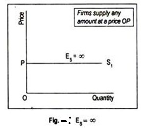
4. Perfectly Elastic Supply (ES = ∞)
The numerical value of elasticity of supply, in exceptional cases, may reach up to infinity. The supply curve PS1 drawn in Fig. has an elasticity of supply equal to infinity. Here the supply curve has been drawn parallel to the horizontal axis. The economic interpretation of this supply curve is that an unlimited quantity will be offered for sale at the price OS. If price slightly drops down below OS, nothing will be supplied.
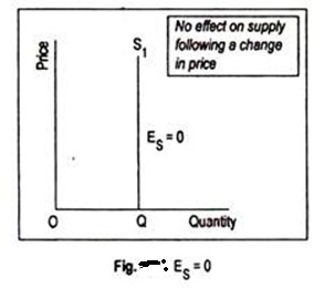
 5. Perfectly Inelastic Supply (ES = 0)
Another extreme is the completely or perfectly inelastic supply or zero elasticity. SS1 curve drawn in Fig. illustrates the case of zero elasticity. This curve describes that whatever the price of the commodity, it may even be zero, quantity supplied remains unchanged at OQ. This sort of supply curve is conceived when we consider the supply curve of land from the viewpoint of a country, or the world as a whole.
Determinants of Elasticity of Supply
Here we are concerned with certain factors which affect elasticity of supply viz., the nature of the good, the definition of the good, the relevance of the time period, and so on.
(a) The Nature of the Good
As with demand elasticity, the most important determinant of elasticity of supply is the availability of substitutes. In the context of supply, substitute goods are those to which factors of production can most easily be transferred. For example, a farmer can easily move from growing wheat to producing jute. Of course, mobility of factors is very important for such substitution.
As a general rule, the more easily the factors can be transferred from the production of one good to that of another, the greater will be the elasticity of supply. Since durable goods can be stored for a long time, its elasticity of supply is very high. But for non-durable goods and perishable goods elasticity of supply tends to be very low.
(b) The Definition of the Commodity
As in the case of demand, elasticity of supply also depends on the definition of the commodity. The narrowly a commodity is defined the greater is its elasticity of supply. For example, it is easier for a tailor to transfer resources from producing red skirts to green skirts than from skirts to men’s trousers.
(c) Time
Time also exerts considerable influence on the elasticity of supply. Supply is more elastic in the long run than in the short run. The reason is easy to find out. The longer the time period, the easier it is to shift resources among products, following a change in their relative prices.
This is usually true in the case of most agricultural commodities, because of the natural time lag between planting and harvesting of crops. In agriculture, production plans have to be made months or even years ahead and they cannot be altered quickly.
(d) The Cost of Attracting Resources
If supply is to be increased it is necessary to attract resources from other industries. This usually involves raising the prices of these resources. As their prices rise, cost of production also increases. So supply becomes relatively inelastic.
If these resources can be obtained cheaply then supply is likely to be relatively elastic. These considerations become very important at times of full employment when the only available factors of production are those which can be attracted from other industries and uses.
(e) The Level of Price
Elasticity of supply is also likely to vary at different prices. Thus, when the price of a commodity is relatively high, the producers are likely to be supplying near the limits of their capacity and would, therefore, be unable to make much response to a still higher price. When the price is relatively low, however, producers may well have surplus capacity which a higher price would induce them to use.
Manufacturing industries, on the other hand, can usually adjust their output upwards or downwards fairly quickly in response to changing conditions in the market.